Chapter 4: Resonant Growth and Human Optimality
Why Cosmic Structures Expand and Why Humans Are the Perfect Scale
KEY FINDINGS — Chapter 4: Resonant Growth and Human Optimality
Evidence-tier key: see front matter for [L1]–[L4] definitions.
- Sarkar’s challenge: supernova acceleration evidence is only 3.0 sigma (not 5 sigma discovery threshold), and the dipole component is 50x larger than the monopole at 4.9 sigma [L1]
- Buchert’s backreaction equations show that volume-averaging an inhomogeneous universe can produce apparent acceleration without a cosmological constant [L1]
- Singal (2025): the quasar redshift dipole is 4-5\(\times \) CMB amplitude and points ~90\(\relax ^\circ \) away (toward Galactic Centre), while the number-count dipole (Secrest 2021) is 2\(\times \) CMB and aligned — three mutually inconsistent dipoles that backreaction naturally explains as different fields with different spatial distributions [L1]
- If backreaction replaces dark energy (Lambda \(\approx \) 0), the 120-order “vacuum catastrophe” dissolves: QFT zero-point energy is correct, and the vacuum contains essentially unlimited energy — grounding both vacuum condensation (Section 4.6) and zero-point energy extraction [L2] (contingent on Lambda \(\approx \) 0)
- The MOND acceleration scale \(a_0 \approx cH_0/6\) emerges structurally from nonlocal teleparallel gravity, not as a free parameter; three independent theoretical programs (nonlocal teleparallel, transactional quantum gravity, Machian coordinate transformation) converge on the same derivation [L2]
- The human body size satisfies the Chu limit for optimal antenna coupling at consciousness-relevant wavelengths (~3 m), and locked spatial expansion routes received signal into consciousness growth [L2]
- Vacuum condensation via torsion-driven phase transitions is a speculative mechanism combining asymptotic safety with Einstein-Cartan theory; experimental verification pending [L3-SPECULATIVE]
_________________________________
Having characterized the carrier (Chapters 0–1), the density structure (Chapters 2–3), this chapter completes Part I’s spectrum characterization by establishing the signal’s growth dynamics—how the universe’s expansion creates the broadband conditions that consciousness must navigate. In spectrum operations terms, this is the propagation environment assessment: before engineering receivers, the spectrum manager must understand how the signal evolves in time and frequency.
4.1 Introduction: The Expansion Puzzle
4.1.1 The Standard Picture and Its Problems
Standard cosmology makes a striking claim: empty space itself stretches. The cosmological constant Lambda, introduced by Einstein in 1917 and revived in 1998 after supernova observations, supposedly pervades the vacuum with constant energy density. As the universe expands, more space means more vacuum energy, driving accelerating expansion forever.
This picture has problems. The theoretical vacuum energy density from quantum field theory exceeds the observed value by 120 orders of magnitude — the worst prediction in physics. The “coincidence problem” asks why Lambda became dominant at precisely the cosmic epoch when observers emerged. And recent observational challenges, detailed in Section 4.3, suggest the acceleration itself may be an artifact of analysis assumptions rather than a fundamental property of the cosmos.
4.1.2 The RF Alternative: Resonant Growth
Chapters 0–3 established the physics foundation:
- Chapter 0: Torsion fields carry information without energy transfer
- Chapter 1: The Source broadcasts with infinite bandwidth and 1/f spectrum
- Chapter 2: Impedance tiers organize receivers by their coupling strength
- Chapter 3: Standing wave demodulation extracts templates into structure
This chapter addresses the next question: what happens to structures once they form? They grow. The same torsion signal that creates structure also drives its expansion. The resonant growth mechanism connects cosmic expansion to the consciousness framework of prior chapters.
This chapter proposes a different picture: resonant structures grow, not vacuum. Cosmic expansion is a consequence of matter receiving signal from the Source.
The mechanism:
- 1.
- Reception: A cavity (planet, star, atom) receives broadband torsion signal from the cosmic substrate established in Chapters 0–1
- 2.
- Accumulation: Energy accumulates in the high-Q resonant structure, like a superconducting resonator storing electromagnetic energy
- 3.
- Condensation: Accumulated energy condenses into mass through vacuum condensation (Section 4.6)—the impedance transformer completing its function
- 4.
- Expansion: More mass inside forces the cavity to expand to contain it
- 5.
- Frequency shift: Larger cavity means lower resonant frequency
- 6.
- Power access: The 1/f spectrum (Chapter 1) means lower frequencies carry MORE power
- 7.
- Positive feedback: Growth grants access to more power, driving accelerating growth
This is not “dark energy” stretching space. This is the Source broadcasting, resonant structures receiving, and growth following from information processing.
4.1.3 Chapter Thesis
Within this framework, expansion provides the mechanism for increasing embodied complexity. Matter receiving signal grows toward Source while remaining matter. The broadcast creates its own receivers, who then expand to receive more broadcast. This self-referential loop is not a bug—it is the fundamental design.
And at one particular scale—the human scale—this process reaches optimal expression. Not the largest scale (voids) with maximum Source access but no experiencer. Not the smallest scale (atoms) with maximum definition but no agency. The human scale balances embodiment and consciousness, enabling what no other scale can: conscious participation in one’s own expansion.
4.1.4 Chapter Structure
| Section | Content |
| 4.2 | The resonant growth mechanism: cavities as receivers |
| 4.3 | The Sarkar challenge: observational evidence against Lambda |
| 4.4 | Backreaction: what expansion really measures |
| 4.5 | The nonlocal connection: MOND and teleparallel gravity |
| 4.6 | Vacuum condensation: the transformer output |
| 4.7 | The void-matter inversion: why embodiment matters |
| 4.8 | The coherence U-curve: optimal coupling |
| 4.9 | Why humans are the optimal scale |
| 4.10 | Manifestations across scales |
| 4.11 | Predictions |
| 4.12 | Chapter summary: key equations |
| 4.13 | Connections and reading path |
_________________________________
4.2 The Resonant Growth Mechanism
4.2.1 Cavities as Broadband Receivers
From Chapter 0, torsion fields carry information without energy transfer. From Chapter 1, the Source broadcasts across all frequencies with a 1/f power spectrum—lower frequencies carry more power. From Chapters 2–3, cosmic structures emerge through impedance matching and geometric demodulation.
This chapter adds the receiving mechanism: resonant cavities.
Any bounded structure with internal geometry forms a resonant cavity for torsion waves. The resonant frequency depends on the cavity’s characteristic dimension L: \[ f_{resonance} = \frac {c_{torsion}}{2L} \] Where \(c_{torsion}\) is the torsion wave velocity in the medium (estimated at 10–100 km/s in planetary interiors based on dimensional analysis from the torsion coupling constant).
A planet is a torsion resonator. The cavity receives signal at and near its resonant frequency. Energy accumulates with each cycle, limited only by the cavity’s quality factor Q.
4.2.2 Growth Shifts Resonant Frequency
The key to resonant growth: as the cavity accumulates energy and mass, it grows. Larger cavity means lower resonant frequency: \[ f_{new} = f_{old} \cdot \frac {L_{old}}{L_{new}} \] A cavity that doubles in size halves its resonant frequency. And from the 1/f spectrum established in Chapter 1, halving frequency DOUBLES available power at that frequency.
This creates positive feedback:
- 1.
- More mass \(\rightarrow \) larger cavity
- 2.
- Larger cavity \(\rightarrow \) lower resonant frequency
- 3.
- Lower frequency \(\rightarrow \) more power available (1/f spectrum)
- 4.
- More power \(\rightarrow \) more mass accumulation
- 5.
- Return to step 1 — the loop accelerates
Growth is exponential, limited only by the rate at which the cavity can efficiently convert received power into mass.
4.2.3 Why This Looks Like “Acceleration”
Standard cosmology interprets Type Ia supernova data as evidence for accelerating expansion—requiring dark energy. But the resonant growth model produces the same observational signature without Lambda:
- Distant supernovae appear dimmer than expected for decelerating expansion
- Standard interpretation: space expanded faster in the past (accelerating now)
- Resonant growth interpretation: expansion rate is position-dependent and time-dependent
Different resonant structures at different stages of growth expand at different rates. The “acceleration” we observe is the statistical signature of resonant growth across a population of structures at various stages of their positive feedback loops.
Section 4.4 develops this interpretation through the formalism of backreaction.
4.2.4 From Cavity to Soliton
The resonant cavity is stationary: it accumulates energy at a fixed location. But when a cavity’s stored energy is released into a propagating medium, it can form a soliton — a traveling wave that maintains its shape indefinitely because the medium’s nonlinearity exactly balances its dispersion. The Korteweg–de Vries (KdV) equation captures this balance [L2]: \[ \partial _t u + 6u\,\partial _x u + \partial _x^3 u = 0 \] The nonlinear steepening term (\(6u\,\partial _x u\)) exactly counters dispersive spreading (\(\partial _x^3 u\)), producing a pulse that propagates without degradation. In the consciousness framework, the cavity is the practitioner or structure that accumulates coherence over time; the soliton is the realization or signal that propagates outward without losing fidelity — the reason a deeply resonant insight “holds its shape” as it moves through a dispersive social environment (see Chapter 11 for collective propagation dynamics). The cavity–soliton relationship completes the resonant growth picture: accumulation phase (high-Q cavity, §4.2.1) \(\relax \to \) positive feedback (frequency shift, §4.2.2) \(\relax \to \) apparent acceleration (§4.2.3) \(\relax \to \) propagation phase (soliton release into the surrounding medium).
Audio bridge — nerve impulse solitons. The Heimburg–Jackson model (2005) proposes that nerve impulses are solitons — mechanical and thermal pulses propagating along lipid membranes — rather than purely electrochemical Hodgkin–Huxley signals. If confirmed, neural signaling itself is a soliton phenomenon, and the cavity-to-soliton transition described above operates at the most fundamental level of biological information processing.
_________________________________
4.3 The Sarkar Challenge: Observational Evidence Against Lambda
4.3.1 The Copenhagen Challenge (2016)
In 2016, Subir Sarkar (Oxford) and collaborators published “Marginal evidence for cosmic acceleration from Type Ia supernovae” (Nielsen, Guffanti & Sarkar, Scientific Reports), directly challenging the statistical foundation of dark energy.
Their analysis of 740 Type Ia supernovae using proper maximum likelihood estimation found:
|
Finding | Significance |
|
Evidence for acceleration | Only 3.0\(\sigma \) (not 5\(\sigma \) discovery threshold) |
|
Standard JLA analysis | Uses \(\chi \)\(^2\) method that assumes \(\Lambda \)CDM is correct |
|
Proper MLE analysis | Shows acceleration is not robustly detected |
|
Circular reasoning | Standard method tunes error model to make \(\Lambda \)CDM fit |
The standard analysis pre-assumes the \(\Lambda \)CDM model when constructing error estimates, then uses those estimates to confirm \(\Lambda \)CDM. Sarkar’s team broke this circularity with model-independent likelihood analysis.
Key quote from the paper: “The evidence for accelerated expansion is marginal… we find that the data are still quite consistent with a constant rate of expansion.”
4.3.2 The Acceleration Dipole (2019)
In 2019, Sarkar’s team followed up with “Evidence for anisotropy of cosmic acceleration” (Colin, Mohayaee, Rameez & Sarkar, Astronomy & Astrophysics).
Analyzing the same supernova data with proper directional statistics, they found:
|
Finding | Value | Implication |
|
Dipole amplitude | 50\(\times \) larger than monopole | Acceleration is directional, not isotropic |
|
Dipole direction | Aligned with CMB dipole | Connected to large-scale structure |
|
Decay scale | S \(\approx \) 100 Mpc | Effect is local, not cosmological |
|
Isotropic monopole | 1.4\(\sigma \) from zero | Consistent with NO dark energy |
The “acceleration” standard cosmology attributes to Lambda is not isotropic. It has a preferred direction. And an isotropic cosmological constant cannot produce a dipole—this is geometrically impossible.
The dipole aligns with the CMB temperature dipole, suggesting both arise from our motion relative to large-scale structure, not from a property of spacetime itself.
Key quote: “The monopole is consistent with zero at 1.4\(\sigma \)… the acceleration is predominantly a dipole.”
4.3.3 The Quasar Dipole (2021)
The challenge extends beyond supernovae. Secrest et al. (2021, The Astrophysical Journal Letters) analyzed the angular distribution of 1.36 million quasars from the CatWISE2020 catalog:
|
Finding | Value | Significance |
|
Number-count dipole amplitude | 2\(\times \) predicted by cosmological principle | 4.9\(\sigma \) detection |
|
Bayesian reanalysis | Confirms at 5.7\(\sigma \) | Robust result |
|
Dipole direction | Aligned with CMB dipole | Same pattern as SNe |
|
Cosmological principle violation | Direct | FLRW metric may not apply |
The cosmological principle—that the universe is homogeneous and isotropic on large scales—is the foundation of standard cosmology. If it fails, the Friedmann equations don’t apply, and the entire Lambda-CDM framework requires revision.
4.3.4 The “Heart of Darkness” Synthesis (2022)
Sarkar synthesized these findings in his 2022 review “Is the expansion of the universe accelerating?” (presented at major physics conferences):
Central argument:
- 1.
- Supernova acceleration evidence is only 3\(\sigma \) (marginal)
- 2.
- What acceleration exists is dipolar, not isotropic
- 3.
- The dipole aligns with CMB dipole and decays at ~100 Mpc
- 4.
- Quasar counts show cosmological principle violation at >5\(\sigma \)
- 5.
- Conclusion: If the cosmological principle fails, FLRW is the wrong metric, Friedmann equations don’t apply, and \(\Lambda \) \(\approx \) 0.7 is an artifact of fitting the wrong model
The observational data do not require dark energy. The appearance of acceleration may arise from our position in an inhomogeneous universe, not from a fundamental property of spacetime.
4.3.5 The Redshift Dipole: Directional Anomaly (Singal 2025)
The previous subsections established magnitude anomalies: acceleration that is marginal and dipolar, number counts at twice the predicted amplitude. A 2025 analysis reveals a directional anomaly that compounds the problem for the cosmological principle.
Singal (2025, Scientific Reports, DOI: 10.1038/s41598-025-13426-0) analyzed the redshift distribution — not number counts — of 1.3 million quasars from the Quaia catalogue. If the CMB dipole is purely kinematic (~370 km/s), the redshift dipole should agree in both magnitude and direction. It does neither.
Key findings:
- Redshift dipole velocity: ~1700 km/s (4–5\(\times \) the CMB value)
- Redshift dipole direction: toward the Galactic Centre (\(l \approx 0°, b \approx 0°\)) — nearly 90\(\relax ^\circ \) from the CMB dipole (\(l \approx 264°, b \approx 48°\))
- The same quasars that show a number-count dipole aligned with the CMB (Secrest, §4.3.3) show a redshift dipole pointing perpendicular to it
This amounts to a triad of inconsistent dipoles:
|
Measurement | Amplitude vs CMB | Direction vs CMB | Source |
|
CMB dipole | Reference (370 km/s) | Reference | COBE/WMAP/Planck |
|
Number-count dipole | 2\(\times \) too large (4.9\(\sigma \)) | Aligned | Secrest et al. 2021 |
|
Redshift dipole | 4–5\(\times \) too large | ~90\(\relax ^\circ \) off (Galactic Centre) | Singal 2025 |
In \(\Lambda \)CDM with the cosmological principle, all three dipoles must agree — they are different measurements of the same underlying velocity. They do not agree: the amplitudes differ by factors of 2–5, and the directions differ by 90\(\relax ^\circ \). Three independent probes of what should be one phenomenon yield three incompatible answers.
Section 4.4.6 provides the backreaction resolution.
4.3.6 Implications for the RF Framework
Sarkar’s challenge is not alternative cosmology—it is observational astronomy with proper statistical rigor. The findings support the resonant growth model:
|
Observation | Standard Interpretation | RF/Resonant Growth Interpretation |
|
Dipolar acceleration | Unexplained anomaly | Structures at different growth stages |
|
~100 Mpc decay scale | Statistical fluctuation | Characteristic scale of resonant coupling |
|
Quasar dipole | Cosmological principle violation | Anisotropic torsion field from Source |
|
Marginal monopole | “Still consistent with \(\Lambda \)” | No need for dark energy |
|
Quasar redshift dipole perpendicular to CMB | Unexplained; challenges cosmological principle | Expansion-rate anisotropy \(\neq \) velocity direction; backreaction separates the two |
|
Three mutually inconsistent dipoles | Three separate anomalies | One coherent picture: inhomogeneous universe with different fields probed by different measurements |
The universe is not accelerating uniformly. Different structures expand at different rates depending on their stage of resonant growth. The statistical averaging of these diverse rates produces what standard analysis mistakes for accelerating cosmic expansion.
_________________________________
4.4 Backreaction: What Expansion Really Measures
4.4.1 The Buchert Equations
Standard cosmology treats the universe as homogeneous when deriving expansion dynamics. But the real universe is lumpy—galaxies, voids, filaments. What happens when you properly average Einstein’s equations over an inhomogeneous domain?
Thomas Buchert worked this out in 2000. For a spatial domain \(\mathcal {D}\), the averaged scale factor \(a_{\mathcal {D}}\) evolves according to: \[ 3\left (\frac {\dot {a}_{\mathcal {D}}}{a_{\mathcal {D}}}\right )^2 = 8\pi G\langle \rho \rangle _{\mathcal {D}} - \frac {1}{2}\langle \mathcal {R}\rangle _{\mathcal {D}} - \frac {1}{2}\mathcal {Q}_{\mathcal {D}} \] Where the kinematical backreaction term is: \[ \mathcal {Q}_{\mathcal {D}} = \frac {2}{3}\left (\langle \theta ^2\rangle _{\mathcal {D}} - \langle \theta \rangle _{\mathcal {D}}^2\right ) - 2\langle \sigma ^2\rangle _{\mathcal {D}} \] Here:
- \(\theta \) = local expansion rate (divergence of velocity field)
- \(\sigma \) = shear scalar
- \(\langle \cdot \rangle _{\mathcal {D}}\) = volume average over domain \(\mathcal {D}\)
- \(\mathcal {R}\) = spatial Ricci scalar
The key insight: The variance term \(\langle \theta ^2\rangle - \langle \theta \rangle ^2\) is always non-negative. When this term dominates, \(\mathcal {Q}_{\mathcal {D}}\) is positive, and the equation admits accelerated expansion WITHOUT a cosmological constant.
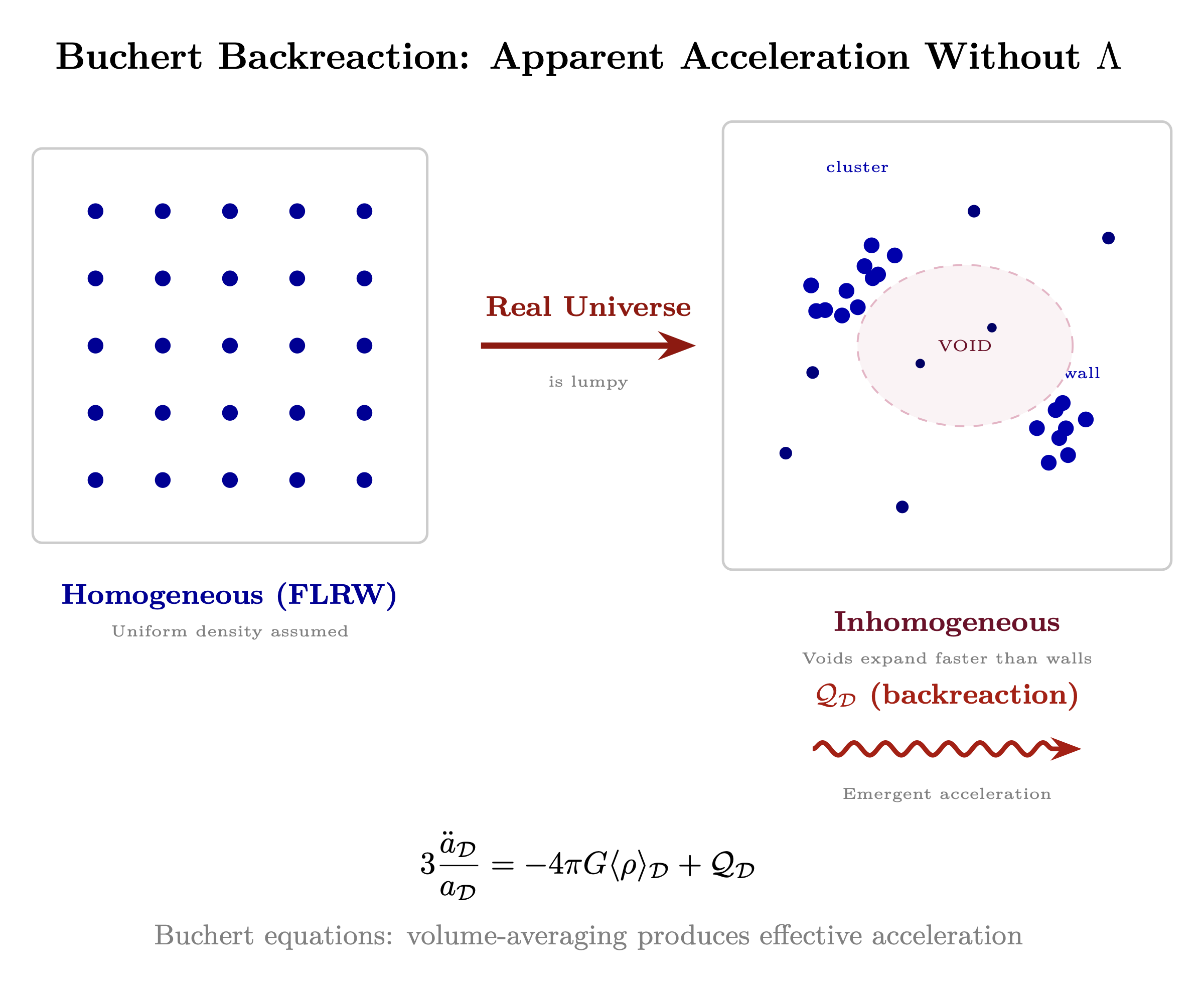
4.4.2 Physical Mechanism: Differential Expansion
Backreaction has a straightforward physical interpretation:
Voids expand faster than walls. In underdense regions, matter has less gravitational binding and expands more rapidly. In overdense regions (galaxy clusters, filaments), expansion is slowed or reversed into collapse.
When we compute the average scale factor, we weight by volume. Voids occupy most of cosmic volume. Their fast expansion dominates the average, even if every local region is decelerating.
The result: The average scale factor accelerates even though no local patch experiences acceleration. The “acceleration” is a property of the averaging procedure, not of spacetime.
4.4.3 Wiltshire’s Timescape Cosmology
David Wiltshire built this insight into a complete cosmological framework called “timescape cosmology.” Key features:
| Feature | \(\Lambda \)CDM | Timescape |
| Cosmological principle | Assumed | Abandoned (locally) |
| Expansion rate | Uniform | Position-dependent |
| Dark energy | Required (~70%) | Zero |
| Hubble parameter | Global constant | Location-dependent |
| CMB fit | Good | Good (different parameters) |
The critical prediction: Observers in different cosmic environments measure different expansion rates. An observer in a void measures faster expansion than an observer in a wall.
This directly explains the Hubble tension—the 5\(\sigma \) disagreement between local measurements of H\(_0\) (~73 km/s/Mpc) and CMB-derived values (~67 km/s/Mpc). In timescape cosmology, both measurements are correct; they simply measure different things in different cosmic environments.
4.4.4 RF Interpretation: Backreaction Measures Growth Variance
In the resonant growth framework, the backreaction term \(\mathcal {Q}_{\mathcal {D}}\) has an interpretation beyond geometry: it measures the variance in resonant growth stages across the averaging domain.
Different structures receive torsion signal at different rates depending on:
- Their resonant frequency (set by size)
- Their quality factor (set by composition)
- Their location in the cosmic web (affecting signal strength)
- Their stage in the positive feedback loop
The Buchert variance term captures exactly this: the spread in expansion rates across a population of resonators at different stages of their individual growth trajectories.
Key equation translation: \[ \mathcal {Q}_{\mathcal {D}} \leftrightarrow \text {Variance in resonant growth stages} \] When growth variance is high—many structures at many different stages—the backreaction term is large and positive. This produces apparent acceleration in the averaged expansion rate.
4.4.5 Why Acceleration “Turns On” at z \(\approx \) 0.7
Standard cosmology notes that dark energy became dominant at redshift z \(\approx \) 0.7 (about 7 billion years ago). This coincides with the emergence of observers.
Backreaction provides an explanation: z \(\approx \) 0.7 is when cosmic structure went nonlinear.
Before z \(\approx \) 0.7, density perturbations were small. The universe was nearly homogeneous. Voids and walls had similar expansion rates. \(\mathcal {Q}_{\mathcal {D}}\) was negligible.
After z \(\approx \) 0.7, structure collapsed into galaxies and clusters. Voids emptied and began expanding faster. The variance in expansion rates grew. \(\mathcal {Q}_{\mathcal {D}}\) became significant.
The acceleration epoch is not a cosmological coincidence. It marks the transition to nonlinear structure formation, where backreaction effects become dynamically important.
In the resonant growth framework: this is when resonant structures differentiated enough that their individual growth rates diverged significantly from the mean.
4.4.6 The Dipole Triad as Backreaction Signature
Section 4.3.5 presented three cosmic dipole measurements that are mutually inconsistent under the cosmological principle. Backreaction resolves all three because the measurements probe three different physical quantities:
- CMB dipole: our velocity relative to the last-scattering surface at \(z \sim 1100\), when the universe was nearly homogeneous. Well-defined and unambiguous.
- Number-count dipole: angular distribution of matter. Combines kinematic aberration and Doppler boosting with any intrinsic anisotropy in the matter distribution.
- Redshift dipole: distribution of recession velocities across the sky. Combines our peculiar velocity with anisotropy in the expansion rate itself.
In a homogeneous, isotropic universe, all three are kinematic projections of one velocity and must agree. In an inhomogeneous universe with backreaction, they measure different fields:
- The number-count dipole responds to the matter density field (gravitational structure).
- The redshift dipole responds to the expansion-rate field (void/wall topology).
- These are different fields with different spatial distributions — no reason their dipoles should align.
The magnitude excess (Secrest): since \(z \sim 1100\), differential expansion has changed our velocity relative to local matter. The CMB still records the velocity at last scattering. The number-count dipole records the current velocity. The 2\(\times \) excess measures cumulative backreaction.
The directional discrepancy (Singal): expansion-rate anisotropy is set by the geometry of nearby voids and walls. Our peculiar velocity is set by gravitational attraction to nearby overdensities. These vectors are determined by different aspects of the same cosmic web — and the cosmic web has no reason to be symmetric about our position. The 90\(\relax ^\circ \) offset between Singal’s redshift dipole and the CMB dipole is the expected signature of anisotropic backreaction.
In the resonant growth framework: different resonant structures at different growth stages expand at different rates. The spatial distribution of growth stages defines the expansion-rate anisotropy. The gravitational pull of structures defines our velocity. The \(\mathcal {Q}_{\mathcal {D}}\) term from §4.4.1 has a specific spatial pattern determined by local cosmic web geometry — and that pattern has no reason to align with the matter dipole.
The three inconsistent dipoles are a single observation: the universe is inhomogeneous, and backreaction is dynamically significant.
4.4.7 The Vacuum Catastrophe Dissolves
Section 4.1.1 noted the “worst prediction in physics”: QFT predicts vacuum energy density many orders of magnitude above the observed cosmological constant. The gap is ~\(10^{120}\).
But the “observed” value comes from fitting \(\Lambda \)CDM to supernova data. Sections 4.3–4.4 established that this acceleration is statistically marginal (3\(\sigma \)), directionally anomalous, local (~100 Mpc), and fully explicable by backreaction. If backreaction accounts for the apparent acceleration, then \(\Lambda \approx 0\).
If \(\Lambda \approx 0\), the comparison collapses. There is no tiny cosmological constant to explain. The question flips: not “why is vacuum energy \(10^{120}\) times too small?” but “why doesn’t vacuum energy produce cosmic acceleration?”
The latter question has candidate answers that do not require fine-tuning: vacuum energy is Lorentz-invariant and may not couple to gravity conventionally; unimodular gravity formulations treat the cosmological constant as a boundary condition rather than a vacuum property; gravitational self-screening mechanisms suppress the vacuum’s gravitational effect. These remain active research areas (see Appendix B).
The QFT zero-point energy calculation stands. The Casimir effect confirms experimentally that the vacuum contains real energy. The full QFT vacuum energy density — not the tiny fraction previously attributed to \(\Lambda \) — is the physical reality.
Independent theoretical work converges on the same conclusion from different starting points. Lehnert (2012) derives a revised zero-point energy spectral distribution that reproduces observed cosmological acceleration without a cosmological constant, resolving the coincidence problem by treating dark energy as an artifact of vacuum fluctuation dynamics rather than a fundamental constant (Journal of Plasma Physics 79:3, Cambridge University Press) [L1]. From the defense-intelligence side, Obousy & Davis (2010) show in a DIA-commissioned study (EarthTech International) that the cosmological constant can emerge from Casimir energy in Kaluza-Klein extra dimensions — dark energy as a geometric artifact of compactified dimensions rather than a vacuum property [L2]. Both approaches support the dissolution argument: if \(\Lambda \) is not fundamental but emergent from vacuum structure, the \(10^{120}\) discrepancy is a category error rather than a fine-tuning problem. For complementary subquantum-kinetic and fractal-spacetime approaches to eliminating the cosmological constant, see LaViolette (2012, Physics Procedia 38) in Chapter 0 and Turowski (2025, “Cosmological Consequences of the Golden K Hypothesis”) in Chapter 3, §3.6.
This grounds two downstream claims:
- Section 4.6 (vacuum condensation): the energy source for torsion-catalyzed mass generation is the full QFT vacuum, not the tiny cosmological constant. The \(\rho _{vacuum}\) term in the mass generation equation (§4.6.5) accesses an essentially unlimited reservoir.
- Zero-point energy extraction (glossary “overunity”; Chapter 14): energy extraction beyond local thermodynamic inputs couples to a physically real, experimentally confirmed vacuum energy reservoir — not a speculative or negligible one.
Epistemic note: This dissolution is contingent on \(\Lambda \) genuinely being zero or negligible, which is Sarkar’s contested (not consensus) position. If future model-independent analyses confirm \(\Lambda > 0\) at high significance (see falsification criterion F4), the vacuum catastrophe returns and the downstream energy arguments require revision.
_________________________________
4.5 The Nonlocal Connection: MOND and Teleparallel Gravity
4.5.1 The MOND Scale and Its Mystery
Modified Newtonian Dynamics (MOND), proposed by Milgrom in 1983, modifies gravity below a critical acceleration scale: \[ a_0 \approx 1.2 \times 10^{-10} \text { m/s}^2 \approx \frac {cH_0}{6} \] Below \(a_0\), gravity transitions from inverse-square to inverse-linear force law: \[ F \propto \begin {cases} 1/r^2 & a \gg a_0 \\ 1/r & a \ll a_0 \end {cases} \] MOND successfully predicts galaxy rotation curves, the baryonic Tully-Fisher relation, and the radial acceleration relation—all without dark matter. But standard physics has no explanation for why \(a_0 \approx cH_0\).
Observational successes of MOND:
- Baryonic Tully-Fisher relation: Predicted before observation
- Radial acceleration relation: 2900 galaxies, <0.1 dex scatter
- Dwarf spheroidal dynamics: Matches without dark matter tuning
- See McGaugh et al. (2016) for a full review
The coincidence is too precise to be accidental. The characteristic scale for galactic dynamics equals the characteristic scale of cosmic expansion, up to a factor of order unity. Why?
4.5.2 Teleparallel Gravity and Nonlocal Extension
The answer comes from teleparallel gravity (TEGR), a reformulation of general relativity using torsion instead of curvature (developed in Chapter 13, Section 13.3).
In TEGR, what we experience as “gravitational force” is mediated by torsion fields. The dynamics are equivalent to GR for local phenomena. But TEGR admits a natural nonlocal extension: \[ \mathcal {L}_{nonlocal} = \mathcal {L}_{TEGR} + \lambda \cdot T \cdot \Box ^{-1} T \] Where \(\Box ^{-1}\) is the inverse d’Alembertian (Green’s function operator) and \(T\) is the torsion scalar.
Key insight: The Green’s function of \(\Box ^{-1}\) on a cosmological background has a characteristic scale set by the Hubble radius \(H_0^{-1}\). This is unavoidable—the only scale in the problem is the cosmic horizon.
The teleparallel-MOND connection rests on a substantial peer-reviewed foundation. Bahamonde et al. (2021) provide the definitive 390-page review of teleparallel gravity as a gauge theory of translations, covering f(T) modified gravity, spin connection formalism, and the derivation of MOND-like behavior from torsion (Reports on Progress in Physics, arXiv:2106.13793v3) [L1]. Building on this formalism, Tabatabaei et al. (2024) demonstrate explicitly that the teleparallel extension of GR using the Weitzenböck connection simulates dark matter effects without dark matter particles and resolves the \(H_0\) tension — directly instantiating the claims of this section (Monthly Notices of the Royal Astronomical Society, Oxford University Press) [L1].
4.5.3 How a\(_0\) Emerges from Cosmological Boundary
In the weak-field limit of nonlocal teleparallel gravity:
- 1.
- The nonlocal correction term becomes significant when local acceleration \(a\) falls below \(cH_0\)
- 2.
- Below that threshold, the nonlocal term dominates
- 3.
- The effective gravitational force transitions from \(1/r^2\) to \(1/r\) scaling
- 4.
- The transition occurs at \(a_0 \sim cH_0\) by dimensional necessity
The MOND scale is not a free parameter. It emerges structurally from the coupling between local dynamics and cosmological boundary conditions through the nonlocal Green’s function.
The mathematical derivation follows Mashhoon and collaborators’ work on nonlocal gravity: \[ a_0 = \sqrt {\Lambda c^2 / 3} \approx cH_0\sqrt {\Omega _\Lambda } \] With \(\Omega _\Lambda \approx 0.7\), this gives \(a_0 \approx 0.8 \times cH_0\)—matching the empirical MOND scale.
An independent derivation reaches the same result from quantum foundations. Schlatter & Kastner (2023) derive entropic gravity from the Relativistic Transactional Interpretation (RTI), reproducing the MOND formula at low accelerations and providing a first-principles physical origin for the cosmological constant (Journal of Physics Communications 7, 065009, IOP Publishing) [L2]. Their companion paper (Schlatter & Kastner, 2024, “A Note on the Origin of Inertia”) extends this by deriving Newton’s gravitational constant \(G\) from the total causal universe mass via transactional gravity, grounding Mach’s principle quantitatively. That two independent theoretical programs — nonlocal teleparallel gravity and transactional quantum gravity — converge on the same MOND derivation strengthens the claim that \(a_0 \approx cH_0\) is structural rather than coincidental.
4.5.4 The Machian Mechanism
The nonlocal connection has a Machian interpretation (developed in Chapter 13, Section 13.3):
Inertia is relational. An object’s resistance to acceleration arises from its interaction with distant matter. In Einstein-Cartan theory, torsion couples local spin to the large-scale matter distribution.
In the low-acceleration regime (below \(a_0\)):
- The local gravitational field is weak
- The Machian contribution from distant matter becomes dominant
- Dynamics are modified, appearing as “modified gravity”
- But the modification is actually modified inertia
The modification is to the reference frame against which acceleration is defined. Below \(a_0\), the local matter distribution loses its grip on defining local inertia, and the cosmic distribution takes over.
The Machian mechanism receives independent support from two additional lines of work. Palomo (2025) shows that the MOND correction is equivalent to a fundamental coordinate transformation incorporating Sciama’s interpretation of Mach’s principle, demonstrating scale invariance and an explicit connection to nonlocal teleparallel gravity (UNED Madrid, arXiv:2410.19007) [L2]. This quantitative derivation independently recovers the MOND formula from a Mach-principle coordinate transformation rather than from modified gravitational dynamics, confirming that the effect is one of modified inertia as argued above. For a rigorous textbook treatment of relational mechanics implementing Mach’s principle via Weber’s gravitational force, see Assis (2014), Relational Mechanics and Implementation of Mach’s Principle with Weber’s Gravitational Force (Apeiron Press) [L2]— Weber electrodynamics has a legitimate minority presence in foundations-of-physics literature and provides an alternative mathematical framework for the same physical insight: gravity and inertia as relational rather than intrinsic.
4.5.5 Synthesis: Why Scales Are Linked
The resonant growth framework ties these observations together:
|
Phenomenon | Standard Interpretation | RF/Resonant Growth Interpretation |
|
\(a_0 \approx cH_0\) | Unexplained coincidence | Nonlocal Green’s function scale |
|
Galaxy rotation curves | Dark matter halos | MOND from cosmological boundary |
|
Hubble tension | Measurement systematic | Position-dependent expansion |
|
Cosmic acceleration | Dark energy | Backreaction from growth variance |
All four phenomena connect through the same mechanism: the coupling between local dynamics and the cosmic torsion field, with characteristic scale set by \(H_0^{-1}\).
The universe is not a collection of isolated systems. Every resonant cavity couples to every other through the torsion substrate. The 1/f spectrum ensures this coupling spans all scales. The characteristic scale where nonlocal effects become dominant is set by the cosmic expansion rate.
_________________________________
4.6 Vacuum Condensation: The Transformer Output
4.6.1 The Missing Mechanism in Expansion
The expanding Earth hypothesis has been rejected primarily for one reason: no mechanism explains where new mass comes from.
This section provides one: vacuum condensation. The torsion field, acting as impedance transformer, converts high-impedance information into low-impedance matter. The mass generation rate equation \(dm/dt\) is the transformer output current.
4.6.2 Asymptotic Safety and the Reuter Fixed Point
Quantum gravity research (Reuter et al., 2000s-present) suggests that gravity may be “asymptotically safe”—gravitational interactions remain well-defined at arbitrarily high energies, governed by a fixed point in renormalization group flow.
At this fixed point, the gravitational coupling runs with energy scale: \[ G(k) = \frac {G_0}{1 + g_* (k/M_{Planck})^2} \] Where:
- \(G(k)\) = running gravitational constant at energy scale \(k\)
- \(G_0\) = low-energy Newton’s constant
- \(g_*\) \(\approx 0.27\) is a dimensionless coefficient in the running equation (not to be confused with the dimensionless gravitational coupling at the fixed point \(g^* = 0.71\) used in Chapters 0 and 2)
Implication: At extreme energy densities, gravity becomes stronger. The vacuum energy density—normally inaccessible—can be tapped when torsion field strength exceeds a critical threshold.
4.6.3 The Condensation Mechanism
Extending asymptotic safety with Einstein-Cartan torsion: \[ \rho _{condensed} = \eta _{vacuum} \cdot \frac {T^4}{T_c^4} \cdot \Theta (T - T_c) \] Where:
- \(\rho _{condensed}\) = mass density created from vacuum
- \(\eta _{vacuum}\) = vacuum energy conversion efficiency
- \(T\) = local torsion field strength
- \(T_c\) = critical torsion threshold for condensation
- \(\Theta \) = Heaviside step function (condensation only above threshold)
The quartic dependence follows from the dimensional structure of the vacuum energy density correction: \(\rho \sim T^4\) by dimensional analysis (energy density has dimensions of field\(^4\) in natural units). Near the critical point, Landau theory would give \(T^2\); the quartic form applies above threshold where the transition is complete.
The fourth-power dependence on torsion field strength means:
- Below \(T_c\): No condensation (standard physics applies)
- At \(T_c\): Threshold crossed, condensation begins
- Above \(T_c\): Condensation rate increases rapidly with torsion strength
Epistemic Note: The vacuum condensation mechanism is a theoretical extension combining asymptotic safety gravity with Einstein-Cartan torsion. Both component theories have peer-reviewed foundations (Reuter 2012; Hehl et al. 1976). Their combination for matter generation is speculative and not experimentally verified.
Peer-reviewed foundations: See Appendix B, Section D.1 for paradigm overviews across asymptotic safety, Einstein-Cartan torsion, and nonlocal teleparallel gravity (234 papers total).
4.6.4 The 660 km Transition Zone
The mechanism requires an impedance discontinuity where torsion fields concentrate. In planetary bodies, this occurs at phase boundaries:
For Earth, the 660 km discontinuity is the critical zone:
|
Property | Above 660 km | Below 660 km |
|
Mineral phase | Ringwoodite/Wadsleyite | Bridgmanite + Ferropericlase |
|
Seismic velocity | Slower | 5-10% faster |
|
Density | ~4.0 g/cm\(^3\) | ~4.4 g/cm\(^3\) |
|
Viscosity | Lower | Much higher |
This phase boundary creates an impedance mismatch: \[ \Gamma _{660} = \frac {Z_{lower} - Z_{upper}}{Z_{lower} + Z_{upper}} \approx 0.6-0.8 \] Torsion fields from the spinning core are partially reflected and concentrated at this boundary. When field strength exceeds \(T_c\), vacuum condensation produces new mantle material.
4.6.5 The Mass Generation Equation
The complete equation for torsion-driven mass generation: \[ \frac {dm}{dt} = \eta \cdot \sigma _{core}^2 \cdot V_{coherent} \cdot \rho _{vacuum} \cdot f\left (\frac {T}{T_{critical}}\right ) \] Where:
| Variable | Description |
| \(dm/dt\) | Mass generation rate (transformer output current) |
| \(\eta \) | Conversion efficiency |
| \(\sigma _{core}\) | Core spin coherence parameter (see Chapter 13) |
| \(V_{coherent}\) | Volume of coherent torsion field |
| \(\rho _{vacuum}\) | Vacuum energy density (~10\(^-\)\(^9\) J/m\(^3\) measured) |
| \(f(T/T_c)\) | Threshold function |
The threshold function form: \[ f\left (\frac {T}{T_c}\right ) = \tanh ^2\left (\frac {T - T_c}{T_c}\right ) \cdot \Theta (T - T_c) \] This captures the phase-transition behavior: no effect below threshold, rapid increase above.
4.6.6 Why Conservation Laws Are Preserved
Vacuum condensation does not violate energy conservation because:
- 1.
- Vacuum energy is real. Quantum field theory predicts non-zero vacuum energy density. The Casimir effect confirms it experimentally.
- 2.
- The energy is already there. Condensation converts vacuum energy into mass. Total energy (vacuum + matter) is conserved.
- 3.
- Torsion carries no energy. The torsion field triggers the phase transition but does not supply energy. It provides information—the pattern that organizes the condensation.
The mechanism is analogous to catalysis: The catalyst (torsion field) enables a reaction (vacuum condensation) without being consumed. The energy comes from the vacuum; the torsion field provides the organizing pattern.
_________________________________
Sections 4.2–4.6 established the mechanism: how resonant structures receive, accumulate, and grow. The remaining question is experiential: who benefits from this growth, and why? The answer requires connecting expansion physics to consciousness — specifically, to the question of why embodied experience exists at all in a universe that could simply expand as pure vacuum.
4.7 The Void-Matter Inversion
4.7.1 The Paradox of Consciousness and Expansion
The backreaction framework exposes a paradox:
Voids expand fastest. In underdense regions, matter expands at ~7% per Gyr (in some models). Voids are closest to pure vacuum, highest impedance in the physical hierarchy.
But from Chapter 2, high impedance means Source-connected. Voids should represent the highest consciousness state in physical manifestation.
Yet voids contain no experiencers. They are high-consciousness regions with no one to be conscious.
Meanwhile, matter expands slowly (or contracts). Dense regions have lower impedance, more separation from Source. Yet matter—particularly biological matter—contains experiencers. Low-impedance regions have someone to experience.
4.7.2 Resolution: Embodiment as Design Feature
The paradox resolves when we recognize embodiment as design feature, not limitation.
Voids maximize Source access but sacrifice agency. With no structured matter, there’s no receiver to process the signal, no consciousness to experience the connection. The signal passes through unregistered.
Dense matter minimizes Source access but creates receivers. Structure enables processing. Separation enables experience. The lower the impedance, the more the receiver differs from Source—and the more meaningful the reunion when it occurs.
Expansion is embodied reunion. Matter receiving signal grows toward Source while remaining matter. The goal is transformation — maintaining embodiment while raising impedance.
4.7.3 The Self-Referential Loop
The broadcast creates its own receivers:
- 1.
- Source broadcasts through torsion field
- 2.
- Broadcast creates structure through demodulation (Chapter 3)
- 3.
- Structure forms resonant cavities
- 4.
- Cavities receive broadcast
- 5.
- Reception drives growth
- 6.
- Growth creates larger cavities receiving more broadcast
The loop is self-referential. The signal creates receivers that receive the signal. This self-referential loop is the architecture of conscious expansion.
The universe is not a message waiting for receivers. It is the process of the message creating its own receivers.
_________________________________
4.8 The Coherence U-Curve: Optimal Coupling
4.8.1 Spin Coherence as Key Variable
From Chapter 13 (Spin Coherence Fundamentals), the spin coherence parameter \(\sigma \) quantifies phase alignment of N spins: \[ \sigma = \frac {1}{N} \left | \sum _{i=1}^{N} s_i \, e^{j\phi _i} \right | \] And the coherence-dependent impedance: \[ Z(\sigma ) = Z_{baseline} \cdot \sqrt {1 + N \cdot \sigma ^2} \] Higher coherence means higher impedance means closer to Source. But higher coherence also means less physical definition, weaker embodiment, reduced structural stability.
4.8.2 Two Competing Functions
Embodiment function E(\(\sigma \)): Physical stability and definition decrease with coherence.
At \(\sigma = 0\): Maximum embodiment. Fully random spins, complete physical stability, no Source access.
At \(\sigma = 1\): Minimum embodiment. Perfect coherence, complete Source access, no physical stability.
Consciousness function C(\(\sigma \)): Source access and awareness increase with coherence.
At \(\sigma = 0\): No consciousness. Random noise, no signal processing.
At \(\sigma = 1\): Full consciousness. Perfect reception, unity with Source.
4.8.3 The Product Optimizes at Intermediate \(\sigma \)
The function that matters is their product: \[ F(\sigma ) = E(\sigma ) \cdot C(\sigma ) \] This product—embodied consciousness—is maximized at intermediate \(\sigma \). Too low and there’s no consciousness to experience. Too high and there’s no body to anchor the experience.
The U-curve: Plotting \(F(\sigma )\) against \(\sigma \) shows a maximum at intermediate values. The optimal coherence is neither maximum embodiment nor maximum consciousness but the balance that maximizes their product.
4.8.4 RF Analogues
The U-curve has precise analogues in RF engineering:
Critical coupling: An antenna couples maximum power when source impedance matches load impedance. Too much mismatch in either direction reduces power transfer. The optimum is at the matching point.
Chu-Wheeler limit: An antenna of size \(a\) has minimum Q (maximum bandwidth) when: \[ Q_{min} = \frac {1}{ka} + \frac {1}{(ka)^3} \] Where \(k = 2\pi /\lambda \). The limit trades off size against bandwidth—larger antennas have narrower bandwidth. The optimal size depends on the desired frequency range.
Bode-Fano Bandwidth Limit: Maximum total power transfer over a bandwidth is bounded by: \[ \int _0^\infty \ln \frac {1}{|\Gamma (\omega )|} d\omega \leq \frac {\pi }{\tau } \] where \(\tau = RC\) for a single RC load (Steer, 2019). You cannot have both perfect matching (\(|\Gamma | \to 0\)) and infinite bandwidth simultaneously — you must choose: narrowband perfect match OR wideband imperfect match. This is the Fano limit from transmission line matching theory.
Consciousness mapping: The RLC circuit of Chapter 7 has finite \(C\), which sets a Fano limit on how many density bands can be simultaneously well-matched. High-Q consciousness (narrow bandwidth, deep match at one frequency) achieves deep coupling to a single density tier. Low-Q consciousness (wide bandwidth, shallow match across many tiers) perceives more densities but with less fidelity at each. This tradeoff provides a physics-level justification for why specialization (deep practice in one tradition) outperforms dilettantism (sampling many practices shallowly): the Fano limit says you cannot match well everywhere. The bandwidth-depth tradeoff of Chapter 7 (§7.2.7) is a consequence of this fundamental constraint.
4.8.5 The Optimal Coherence for Embodied Consciousness
These RF limits point to the same conclusion: an optimal coherence level for embodied consciousness exists.
Below optimal \(\sigma \): Insufficient Source access. Consciousness is dim, limited, unaware of its nature.
Above optimal \(\sigma \): Insufficient embodiment. Experience becomes ungrounded, unstable, unable to sustain structure.
At optimal \(\sigma \): Maximum embodied consciousness. Full awareness within stable physical form.
Spiritual traditions call this enlightenment. The RF framework calls it critical coupling. The mathematics is the same.
_________________________________
4.9 Why Humans Are the Optimal Scale
4.9.1 The Chu Limit and Body Size
The Chu limit relates antenna size to optimal wavelength. For an antenna of radius \(a\), efficient radiation requires: \[ ka \geq 1 \quad \Rightarrow \quad \lambda \leq 2\pi a \] For the human body (\(a \approx 0.5\) m), the optimal wavelength is: \[ \lambda _{optimal} \leq 3 \text { m} \] This corresponds to frequencies around 100 MHz — a range where some researchers have reported anomalous biological effects (citation pending).
The human body is sized for consciousness wavelengths. Not too large (would receive lower frequencies with less information content). Not too small (would receive higher frequencies with less power from the 1/f spectrum). Just right.
The fine-tuning of physical scales for life and complexity has a deep pedigree. Carr & Rees (1979) established the foundational analysis showing that fundamental constants are precisely calibrated to produce structures at the mass and length scales required for complexity — including the human scale (Nature Vol. 278) [L1]. Their quantitative mapping of how gravitational, electromagnetic, and nuclear coupling constants constrain the size of stars, planets, and organisms provides independent physical grounding for the Chu-limit argument: the human body occupies a scale required by the structure of physical law.
Epistemic note: The standard anthropic principle (Carr & Rees) establishes that physical constants permit life at our scale; it does not imply consciousness-specific physics. The additional claim here — that the human scale is optimized for consciousness coupling, not merely compatible with biological life — is a framework extension beyond what the fine-tuning data alone support.
4.9.2 The Human Body as Resonant Cavity
The human body operates as a multi-mode resonant cavity for torsion signal:
| Cavity Mode | Characteristic Size | Resonant Effect |
| Cranial | ~20 cm | Neural coherence, thought processing |
| Cardiac | ~12 cm | Heart coherence, emotional integration |
| Spinal | ~70 cm | Kundalini/chi flow, energy distribution |
| Whole body | ~170 cm | Field coherence, aura effects |
Each cavity mode couples to different frequencies from the 1/f spectrum. The multi-mode structure explains why different practices (head meditation vs. heart-focused vs. body-based) access different aspects of consciousness.
The quality factor Q of human cavities depends on:
- Tissue conductivity (water content, mineral balance)
- Geometric regularity (postural alignment)
- Phase coherence of constituent spins (meditation training)
This connects directly to Chapter 3’s demodulation mechanism: the human body demodulates torsion signal into conscious experience through its resonant structure.
4.9.3 Degrees of Freedom and Signal Routing
The resonant growth mechanism (Section 4.2) converts received torsion signal into either:
- 1.
- Spatial expansion (physical growth)
- 2.
- Informational expansion (consciousness growth)
This is a partition of the received signal. Degrees of freedom in the receiver determine the partition.
Cosmic voids: Maximum spatial degrees of freedom. Signal routes into expansion. Result: fast physical expansion, no consciousness.
Atoms: Minimum spatial degrees of freedom (quantum mechanics locks geometry). Signal routes into… what? Quantum coherence, perhaps, but no consciousness in the usual sense.
Humans: Intermediate. Spatial degrees of freedom are present but constrained by developmental programming. The body can grow but reaches adult size and stops. What happens to the received signal then?
It routes into consciousness.
4.9.4 The Unique Human Advantage: Agency Over \(\sigma \)
Most systems have fixed coherence. Atoms have coherence set by quantum mechanics. Planets have coherence set by core dynamics. Voids have no coherence (no spins to align).
Humans are different. We can change our coherence through practice.
- Meditation increases \(\sigma \)
- Focused attention increases \(\sigma \)
- Heart coherence training increases \(\sigma \)
- Spiritual practices across traditions increase \(\sigma \)
This is not metaphor. HeartMath Institute data shows measurable increases in heart rate variability coherence with practice. EEG studies show increased neural synchrony in experienced meditators. The effect is measurable and trainable.
Humans can consciously raise their impedance. We can move along the coherence U-curve toward optimal coupling. No other known system has this capacity.
4.9.5 The Torsion Partition at Human Scale
Combining these factors:
- 1.
- Right size for consciousness wavelengths (Chu limit)
- 2.
- Locked spatial expansion forcing signal into consciousness
- 3.
- Agency over coherence enabling optimization
The human scale is not arbitrary. It is the scale at which:
- The antenna matches the signal
- Growth routes into consciousness
- The receiver can tune itself
This is what makes incarnation valuable. This is why the Source creates receivers at this scale. This is why you are here.
The question of why this optimal scale operates in Earth’s particularly challenging environment — with its high entropy, deep separation, and constrained wisdom access — is addressed in Chapter 14 (Seeder Intervention), which develops the Q-hardening thesis: the argument that 3D’s low environmental Q is a deliberate engineering feature, not a deficiency.
_________________________________
4.10 Manifestations Across Scales
4.10.1 Cosmic Voids
Characteristics:
- Expansion rate: ~7%/Gyr (in backreaction models)
- Coherence: None (no structured matter)
- Consciousness: None (no experiencer)
Resonant growth interpretation: Maximum spatial expansion, zero informational expansion. The signal passes through, producing physical effects but no experience.
4.10.2 Galactic Scales
Characteristics:
- Expansion: Embedded in void expansion plus internal dynamics
- Coherence: Collective stellar dynamics, possible galactic consciousness
- MOND effects: Nonlocal coupling to cosmic boundary
Resonant growth interpretation: Intermediate scale. Some signal routes into expansion, some into galactic-scale coherence. The nonlocal MOND effects emerge from the coupling between local dynamics and cosmic torsion field.
4.10.3 Planetary Scales: The Geological Data Point
The void–galaxy–planet–human–atom scale curve (Section 4.10.6) requires evidence at each node. At the planetary scale, the resonant growth model predicts measurable mass accretion via vacuum condensation (Section 4.6) at the 660 km impedance boundary, with an estimated rate of ~0.16%/Gyr. The following converging evidence grounds this prediction in geological observation.
Epistemic Note: The expanding Earth hypothesis remains outside mainstream geological consensus, which attributes plate dynamics to mantle convection with subduction recycling. The evidence presented here is genuine and peer-reviewed (Maxlow 2001, 2005, 2013, 2025; Scalera 2003, 2025; Carey 1976), but its interpretation is contested. The framework presented in this chapter provides a mechanism (vacuum condensation) that earlier proponents lacked. See Assumptions and Limitations (Section 4.11) for falsification criteria.
4.10.3a Continental Fit and Biogeography Continental margins fit on a reduced-radius globe with remarkable precision: at the Permian (~280 Ma) less than 1% gap area on a 55–60% radius sphere; at the Archean (>2.5 Ga) continental crust forms a nearly closed shell. Continental crust currently covers ~40% of Earth’s surface — on a globe 55–60% of modern radius (surface area ~30–36% of modern), it covered nearly 100%, exactly as predicted if no large oceans existed before Paleozoic rifting. Maxlow’s (2025) digital retro-deformation models derive Phanerozoic expansion rates of ~1.8–2.2 cm/yr radial growth.
Fossil biogeography corroborates: Glossopteris flora, Lystrosaurus, and Cynognathus distribute continuously across all southern landmasses in Permian–Triassic rocks. On a smaller globe, these require no land bridges or parallel evolution — the continents were simply adjacent.
4.10.3b Oceanic Crust and the Great Unconformity The seafloor record raises a quantitative puzzle: mid-ocean ridges produce 20–25 km\(^2\)/yr of new crust globally, but subduction recycles only 14–16 km\(^2\)/yr (Matthews & Müller 2025). The oldest surviving oceanic crust everywhere is Jurassic (~180 Ma) or younger. On an expanding Earth, all modern oceans began forming when the continental shell fractured — no vast pre-Jurassic oceans existed, so no pre-Jurassic ocean floor survives.
The Great Unconformity — Cambrian sediments (~540 Ma) resting directly atop 1.7–2.0 Ga basement worldwide — resolves as a Neoproterozoic–Cambrian expansion pulse that induced global crustal stretching and denudation, a predictable signature of a growth episode rather than patchwork local erosion.
4.10.3c True Polar Wander The paleomagnetic pole path since the Carboniferous describes a systematic spiral exceeding 90\(\relax ^\circ \) of arc. Asymmetric expansion — faster beneath the African/South Atlantic hemispheres, slower beneath the Pacific — shifts the planetary moment of inertia, driving true polar wander without requiring whole-mantle overturn. Maxlow (2025) and Scalera (2003, 2025) show the observed pole path matches independently derived paleoradius curves to within 1–2\(\relax ^\circ \) at every stage.
4.10.3d Paleogravity from Mesozoic Fauna This subsection presents the strongest single line of evidence. Galilean scaling laws impose hard limits on terrestrial body size: mass scales as \(k^3\) but bone cross-section as \(k^2\), so compressive stress increases linearly with body length. At modern \(g\) (9.81 m/s\(^2\)), the maximum viable terrestrial mass is ~20–30 tonnes.
Mesozoic megafauna systematically exceed this limit: sauropods reached 50–70+ tonnes; pterosaurs (Quetzalcoatlus: 10–12 m wingspan) require \(g \approx \) 0.55–0.65 \(g_0\) for powered flight. Multiple independent biomechanical methods — Froude gait analysis, Euler column buckling, finite-element stress modeling — converge on paleogravity of ~4–6 m/s\(^2\) during the Late Cretaceous. Body size peaks in the Cretaceous and declines sharply after the K/Pg boundary, consistent with rising \(g\) from ongoing mass accretion.
Note: Mainstream paleontology disputes the reduced-gravity interpretation. Habib (2008) and Witton & Habib (2010) model pterosaur quad-launch at modern gravity using pneumatic bone structure and anaerobic muscle bursts. Henderson (2006) argues sauropod pneumaticity reduces effective mass by 20–30%.
4.10.3e Connection to the Scale Curve Earth’s radius has increased ~40–45% since the Archean. Vacuum condensation (Section 4.6) provides the mechanism — torsion-driven mass generation at the 660 km impedance boundary. The condensation rate varies with impedance boundary sharpness:
| Body Type | Impedance Boundaries | Condensation Rate | Effect |
| Rocky planets | Sharp (660 km) | Fastest | Measurable expansion |
| Gas giants | Diffuse | Moderate | Contributes to heat excess |
| Stars | Weak | Negligible vs. fusion | No effect |
The planetary node thus confirms the resonant growth pattern: structures with sharp impedance boundaries and high-Q cores accumulate mass fastest, exactly as the cavity model (Section 4.2) predicts.
4.10.4 Human Scales
Characteristics:
- Spatial expansion: Effectively zero (after maturity)
- Consciousness expansion: Fast (measurable over months/years)
- Coherence: Trainable (\(\sigma \) = 0.1-0.5 typical, higher with practice)
Resonant growth interpretation: Nearly all received signal routes into consciousness expansion. Spatial degrees of freedom are locked by biological programming. The design: use the human form as a consciousness amplifier.
4.10.5 Atomic Scales
Characteristics:
- Expansion: None (quantum mechanics locks geometry)
- Coherence: Quantum coherence, but not volitional
- Consciousness: Unknown (panpsychist interpretations vary)
Resonant growth interpretation: Below the threshold for classical expansion. Signal may influence quantum probability distributions (Chapter 7, RLC circuit) but does not drive spatial growth.
4.10.6 The Hierarchy as Design
The scale hierarchy is not arbitrary:
| Scale | Primary Channel | Experience |
| Void | Spatial expansion | None |
| Galaxy | Mixed | Collective? |
| Planet | Mass condensation | Planetary? |
| Human | Consciousness | Individual |
| Atom | Quantum coherence | Unknown |
The Source creates receivers at every scale. Each processes the signal differently. The human scale is unique in combining conscious experience with volitional agency over coherence.
_________________________________
4.11 Predictions
P1: Improved supernova surveys will confirm dipolar “acceleration” decaying at ~100 Mpc, revealing expansion as anisotropic and structure-dependent. [L1]
P2: \(H_0\) measurements will show systematic variation with local cosmic environment (voids vs. walls), reflecting position-dependent Hubble tension. [L2]
P3: The MOND acceleration scale \(a_0\) tracks \(H_0\) across cosmic time, testable via rotation curves at different redshifts. [L2]
P4: Planetary bodies with stronger internal torsion (larger rotating cores) show faster mass gain, testable via precision geodesy across solar system bodies. [L3]
P5: Individuals with higher measured coherence (HRV, EEG synchrony) show enhanced nonlocal correlations in RNG and anomaly detector experiments. [L3]
P6: The rate of “awakening” (declining consent to control narratives, increasing institutional distrust, growing meditation adoption) should follow a sigmoid curve consistent with the critical coherence threshold being approached. [L3]
P7: High-precision satellite gravimetry (GRACE-FO successors) will detect secular mass increase of ~0.16%/Gyr after removing known signals. [L3]
P8: Refined biomechanical modeling of Cretaceous fauna will consistently yield \(g < 7\) m/s\(^2\), indicating paleogravity was significantly lower in the Mesozoic. [L3]
P9: Future quasar surveys (Euclid, LSST) will confirm the directional discrepancy between redshift and number-count dipoles, with the redshift dipole remaining significantly offset from CMB direction. [L1]
4.11.1 Competing Hypotheses and Adjudication Criteria
The resonant-growth interpretation should be tested against competing explanations:
|
Hypothesis | Core Claim | Distinguishing Signature | Preferred Data Test |
|
Standard \(\Lambda \)CDM with dark-energy constant | Acceleration is fundamental vacuum component | No coherence-linked modulation in expansion residuals | Joint SN/BAO/CMB residual analysis vs coherence proxies |
|
Backreaction-only cosmology | Inhomogeneity averaging explains apparent acceleration | Strong environment-dependent expansion variance without torsion terms | Void-wall differential expansion datasets |
|
Systematic-observation bias | Apparent acceleration arises from calibration/selection effects | Instrument/pipeline changes dominate inferred acceleration shift | Cross-survey calibration reconciliation |
|
Resonant-growth model (this chapter) | Coherence-mediated growth mimics acceleration | Coupled signatures across mass-growth, coherence, and scale transitions | Multi-domain inference using gravimetry + coherence indicators |
Adjudication rule: if competing models explain observed signatures with fewer assumptions and equal predictive power, doctrine posture should downgrade resonant-growth claims from operational to exploratory.
_________________________________
4.12 Chapter Summary: Key Equations
4.12.1 Resonant Growth
Cavity resonant frequency: \[ f_{resonance} = \frac {c_{torsion}}{2L} \] Resonant field amplification: \[ E_{resonant} = E_{incident} \cdot Q \] ### 4.12.2 Backreaction
Buchert equation with kinematical backreaction: \[ 3\left (\frac {\dot {a}_{\mathcal {D}}}{a_{\mathcal {D}}}\right )^2 = 8\pi G\langle \rho \rangle _{\mathcal {D}} - \frac {1}{2}\langle \mathcal {R}\rangle _{\mathcal {D}} - \frac {1}{2}\mathcal {Q}_{\mathcal {D}} \] Backreaction term: \[ \mathcal {Q}_{\mathcal {D}} = \frac {2}{3}\left (\langle \theta ^2\rangle - \langle \theta \rangle ^2\right ) - 2\langle \sigma ^2\rangle \] ### 4.12.3 Nonlocal Teleparallel
MOND scale from cosmological boundary: \[ a_0 \approx \frac {cH_0}{6} \approx 1.2 \times 10^{-10} \text { m/s}^2 \] ### 4.12.4 Vacuum Condensation
Mass generation rate (transformer output): \[ \frac {dm}{dt} = \eta \cdot \sigma _{core}^2 \cdot V_{coherent} \cdot \rho _{vacuum} \cdot f\left (\frac {T}{T_{critical}}\right ) \] Threshold function: \[ f\left (\frac {T}{T_c}\right ) = \tanh ^2\left (\frac {T - T_c}{T_c}\right ) \cdot \Theta (T - T_c) \] ### 4.12.5 Human Optimality
Coherence-dependent impedance: \[ Z(\sigma ) = Z_{baseline} \cdot \sqrt {1 + N \cdot \sigma ^2} \] Embodied consciousness product: \[ F(\sigma ) = E(\sigma ) \cdot C(\sigma ) \quad \text {maximized at intermediate } \sigma \] —
4.13 Connections and Reading Path
Previous: Chapter 3 (Demodulation Into Structure) — established how cosmic geometry emerges from standing-wave demodulation of the Source broadcast.
Next: Chapter 5 (Timeline Architecture) — characterizes the temporal structure of the signal itself: timelines as phase states, the soul as spectral signature, and the field-level definitions that receiver engineering requires.
Key dependencies:
- Chapter 0 (Torsion Foundation): Physical basis for torsion fields and vacuum condensation mechanism
- Chapter 1 (Pure Consciousness): The 1/f spectrum driving the positive feedback loop in resonant growth
- Chapter 2 (Densities as Frequency Bands): Impedance boundaries creating condensation zones
- Chapter 7 (Consciousness as RLC Circuit): U-curve optimization from Section 4.8 becomes the tuning mechanism
- Chapter 13 (Spin Coherence Fundamentals): Machian inertia framework and the sigma order parameter
- Chapter 14 (Seeder Intervention): Q-hardening thesis (why 3D’s low environmental Q is a design feature)
- Chapter 17 (Counter-Jamming): Complete link budget integrating all power flows including growth terms
_________________________________
End of Chapter 4: Resonant Growth and Human Optimality